Exponential Regression using Newton’s Method

We now show how to create a nonlinear exponential regression model using Newton’s Method.

Property 1: Given samples {x₁, …, x_n} and {y₁, …, y_n} and let ŷ = αe^βx, then the value of α and β that minimize $sum{}$ (y_i − ŷ_i)² satisfy the following equations:

Proof: For a proof using calculus, click here

Property 2: Under the same assumptions as Property 1, given initial guesses α₀ and β₀ for α and β, let F = [f g]^T where f and g are as in Property 1 and

Now define the 2 × 1 column vectors B_n and the 2 × 2 matrices J_n recursively as follows

Then provided α₀ and β₀ are sufficiently close to the coefficient values that minimize the sum of the deviations squared, then B_n converges to such coefficient values.

Proof: For a proof using calculus, click here

Property 3: The approximate covariance matrix for the coefficients vector is given by

where

Example 1: We now show how to calculate the value of the α and β coefficients for the exponential regression model for the data in Example 1 of Exponential Regression using a Linear Model or Exponential Regression using Solver (repeated in range A3:B14 of Figure 0), this time using Newton’s Method (i.e. Property 2).

Exponential regression Solver output

Figure 0 – Data for Example 1

The first 5 iterations of Newton’s method are shown in Figure 1. As you can see the coefficients calculated in step 5 (range B31:B32) are the same as those in step 4 (range B28:B29) and so convergence is reached after 5 steps, with values α = 12.50475 and β = .016854.

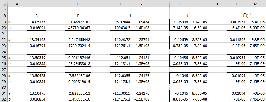
Exponential regression Newton's Method

Figure 1 – Exponential Regression using Newton’s Method

In Figure 2 we show key formulas used in Figure 1 based on Property 1 and 2 and referencing the input X data in range A4:A14 and Y data in range B4:B14 from Figure 1 of Exponential Regression using Solver.

Item	Cells	Formula
B₀	B19:B20	use values from Excel exponential regression
F₀	D19	=SUMPRODUCT(SUMPRODUCT($B$4:$B$14-B19EXP(B20$A$4:$A$14),EXP(B20*$A$4:$A$14)))
F₀	D20	=B19SUMPRODUCT(SUMPRODUCT($B$4:$B$14-B19EXP(B20$A$4:$A$14),EXP(B20$A$4:$A$14),$A$4:$A$14))
J₀	F19	=-SUMPRODUCT(EXP(2B20$A$4:$A$14))
	G19	=SUMPRODUCT(SUMPRODUCT($B$4:$B$14-2B19EXP(B20$A$4:$A$14),EXP(B20$A$4:$A$14),$A$4:$A$14))
	F20	=G19
	G20	=B19SUMPRODUCT(SUMPRODUCT($B$4:$B$14-2B19EXP(B20$A$4:$A$14),EXP(B20*$A$4:$A$14),$A$4:$A$14^2))
J₀^-1	I19:J20	=MINVERSE(F19:G20)
B₁	B22:B23	=B19:B20-MMULT(I19:J20,D19:D20)

Figure 2 – Formulas from Figure 1

We can now create the regression analysis as shown in Figure 3.

Exponential regression results Newton

Figure 3 – Exponential Regression results using Newton’s Method

Key formulas are shown in Figure 4, referencing the cells in Figure 1.

Item	Cells	Formula
α coefficient	P25	=B31
β coefficient	P26	=B32
α s.e.	Q25	=SQRT(L31*R21)
β s.e.	Q26	=SQRT(M32*R21)
SSE	Q21	=SUMPRODUCT((B4:B14-B31EXP(B32A4:A14))^2)
MSE	R21	=Q21/P21

Figure 4 – Formulas from Figure 3

Observation: The following is an alternative approach for finding the regression coefficients α and β. By Property 1

Thus, if α ≠ 0 we can solve for α to get

Thus the original two equations in two unknowns can be replaced by the following equation in one unknown:

This can be solved iteratively using Newton’s Method in one variable, as described in Newton’s Method.

Observation: There is another algorithm that is commonly used to find the regression coefficients called the Levenberg-Marquardt algorithm, which combines the advantages of Newton’s Method with those of the algorithm used by Solver. We won’t consider this algorithm further here.

Related posts: